pynari (Ray Traced ANARI rendering in Python) – First Light!

I haven’t written much for a while – partly because I was too busy, partly because some of the stuff i worked on I couldn’t write about, and mostly, because much of the stuff that I could in theory write about wasn’t exactly “ready enough” to do so. Much of that is now slowly falling into place, though, so it’s about time I start writing some of them up.

Let’s start with pynari (https://pypi.org/project/pynari/) : for those that already know what ANARI is that name will be an immediately recognizable play on two different words – the "py" comes from python, obviously, and the “nari” comes from ANARI…. and that’s exactly what it is: a python-interface for the ANARI ray traced rendering API (including a OptiX/NVIDIA GPU accelerated renderer implementing that API), all installable through pip, and really easy to use from python in a way similar to this:

pip install pynari

then in python:

import pynari as anari

device = anari.newDevice('default')
# create the world:
mesh = device.newGeometry('triangles')
...
world = device.newWorld()
...
world.setParameterArray('surface', anari.SURFACE, ...) 
...
frame.setParameter('world',world)
# render a frame:
frame.render()
fb_color = frame.get('channel.color')

(for some complete, ready-to-run samples look here: https://github.com/ingowald/pynari).

ANARI

If you already know what ANARI is (you should!), then the above should be instantly recognizable, and you’ll probably be able to write some ANARI code in python right away. For those that don’t (yet?) know about ANARI, let’s first rectify this.

ANARI is a fairly recent effort by the Khronos group (the guys that are also spec’ing OpenGL, OpenCL, and all other kind of cross-platform things) to standardize an API for “analytical rendering”. Now I’m not entirely sure what “analytical” is really supposed to mean, so let’s just call it by another name: it’s a ray tracing rendering API, plain and simple, roughly based on the same concepts that were originally used in Intel’s OSPRay API (more info on that here: https://www.ospray.org/talks/IEEEVis2016_OSPRay_paper_small.pdf). In particular, compared to the more widely known ray tracing APIs like OptiX, DXR, or Vulkan, the API level in ANARI is “one step higher” : you don’t have a low-level API that traces individual rays (with you having to write the renderer), but instead, the ANARI API is a ray tracing rendering API, where you create a “world”, populate it with “surfaces”, “volumes”, “lights”, etc, and eventually ask it to render a “frame”. You don’t have to be a ray tracing expert (you probably don’t even have to know how it works at all!), you just set up the world, and ask it to render images. For those interested in the official ANARI 1.0 spec – and/or the official SDK – please look here https://registry.khronos.org/ANARI/specs/1.0/ANARI-1.0.html and here https://github.com/KhronosGroup/ANARI-SDK .

PY-NARI

Anyway, back to pynari. The group of users most benefitting from the ANARI API is, of course, group of people that want to use ray tracing, but that do not necessarily want to become experts in writing their own renderers. Having said that, I eventually realized that this description would probably also – and maybe even in particular – fit python users: many python users (in my experience) tend to be really good at just using libraries/packages that do the heavy work (often in native C/C++/CUDA code)… avoiding the need to become experts in whatever is going on inside that package, as long as it has a nice “pythonic” way of accessing its goodies. (C/C++ users instead tend to be the opposite, generally preferring to re-implement each API for themselves “just because” …. well, guilty as charged, i guess :-/ ).

So, having realized that ANARI should in theory be pretty useful to at least some python users (there just must be some folks out there that wants to do generate some ray traced images in python!) the next task was to figure out how to make that accessible to such users – enter pynari. The first decision I made was to write my own python interface (said pynari): the ANARI SDK already does provide some low-level python bindings, but these only expose the C99 API, and I didn’t think that that was sufficiently “pythonic” for the typical python user. As such, for pynari I took the liberty of slightly deviating from the C API, and instead adopted a much more object-oriented API (which actually fits ANARI very well, because ANARI itself is all about different “objects” that jointly describe what is to be rendered). For example, what in the official C-99 interface looks like this:

ANARILibrary library = anariLoadLibrary("default",...);
ANARIDevice device = anariNewDevice(library,...);
anariCommitParameters(device,device);
ANARICamera camera
  = anariNewCamera(library,device,"perspective");
anariSetParameter(device, camera, 'aspect', 
                  ANARI_FLOAT32, width/height)...

… in pynari becomes what I’d consider more pythonic like this:

import pynari as anari
device = anari.newDevice('default')
camera = dev.newCamera('perspective')
camera.setParameter('aspect',anari.FLOAT32,width/height)

etc.

For “bulk” data like vertex or index arrays, volume voxel data, etc, I decided to mostly build on numpy – i.e., you’d load/create/manipulate the bulky data in numpy, then create an anari “array” wrapper, and use that:

vertex = np.array(....,dtype=np.float32)
array = anari.newArray(anari.FLOAT32,vertex)
mesh.setParameter('vertex.position',array)

Other than slightly adapting the API to look more pythonic, the second big “digression” from the true path of ANARI I made is to – at least for now – hard-bake a single backend implementation into the pynari pip-wheels: In theory, the ANARI API is supposed to be “abstract” in the sense that Khronos only specifies the API itself, so different vendors/developers can each provide their own implementations for it. In your ANARI application, the first thing you’d then do is specify which implementation you want by “loading” a specific “library” (say “ospray” if you’re on a CPU, or “barney” or “visrtx” if you have a RTX-capable GPU, etc). The problem with that is that this multi-backend thing makes the building of the python wheels annoyingly tricky, because you’d have to build all these different backends into the same python wheel – and though it’s probably “possible” to do that it certainly ain’t for the faint of heart (it’s already rather non-trivial, believe you me!). So, while I’m absolutely not trying to make a vendor-independent API vendor-specific on python, at least for now pynari has a single working back-end (and for those wondering, it’s obviously my “barney” GPU renderer). Consequently, to run the pynari that’s currently up on PyPI you currently need a RTX-capable NVIDIA GPU (Turing or newer, data center GPUs most certainly included!). If you have one of those, however, you should now be able to pip-install pynari on either Windows (python 3.12 or 3.13) or Linux (3.9 and newer).

Volunteers, one step forward!

Long story short: on either Windows or Linux, you should by now be able to simply do

pip install pynari

and then run any of the examples I’ve been providing on the pynari github repo (https://github.com/ingowald/pynari)… and of course, you should be able to modify these examples, add to them, write new ones, etc.

Fair warning: this really is “first light” for this package – the backend (barney) has now been used for quite a few different things, but pynari itself is still very “hot off the press”, and “not much tested”. I’m fairly sure there’ll be missing or broken things in there, and I’d certainly expect quite a few “hard aborts” if you do something in a way that isn’t supported yet. That said, I can’t be fixing things I don’t know about, so what I’m looking for is a set of adventurous “volunteers” that would be interested in at least playing with it. Install it, run it, let me know how it goes – send me an email, file an issue on github, comment to this post, … any feedback is useful. Extend some of the samples (I’d particularly like one that’d create a better test volume for the volume rendering sample!), or write your own samples, etc – let me know. And if you create some additional samples, I’d be happy to share them, either here or on the github repo. Any feedback is useful!

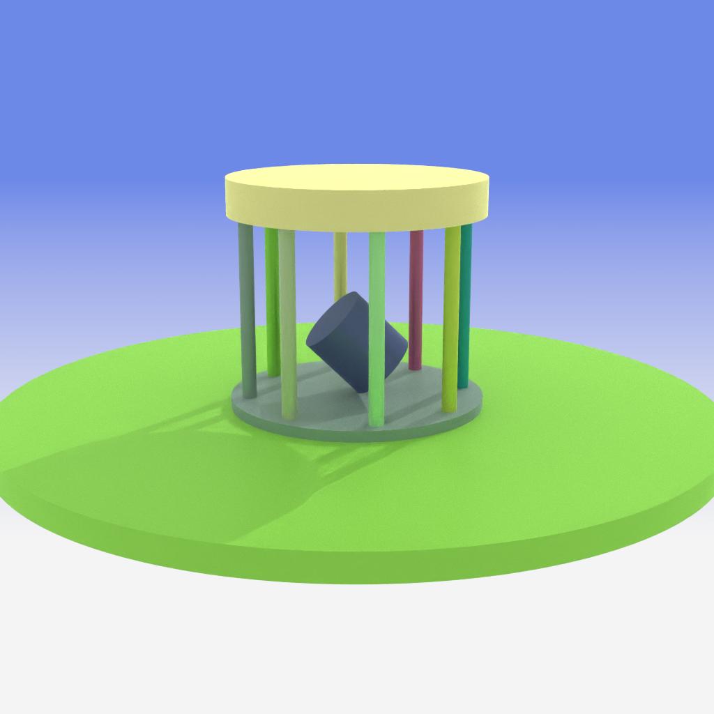
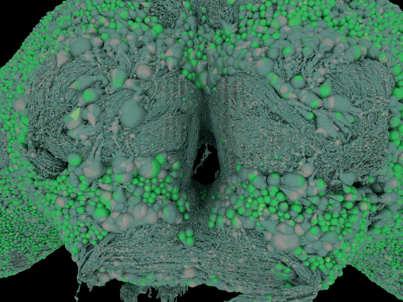
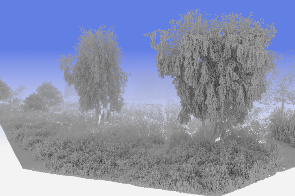
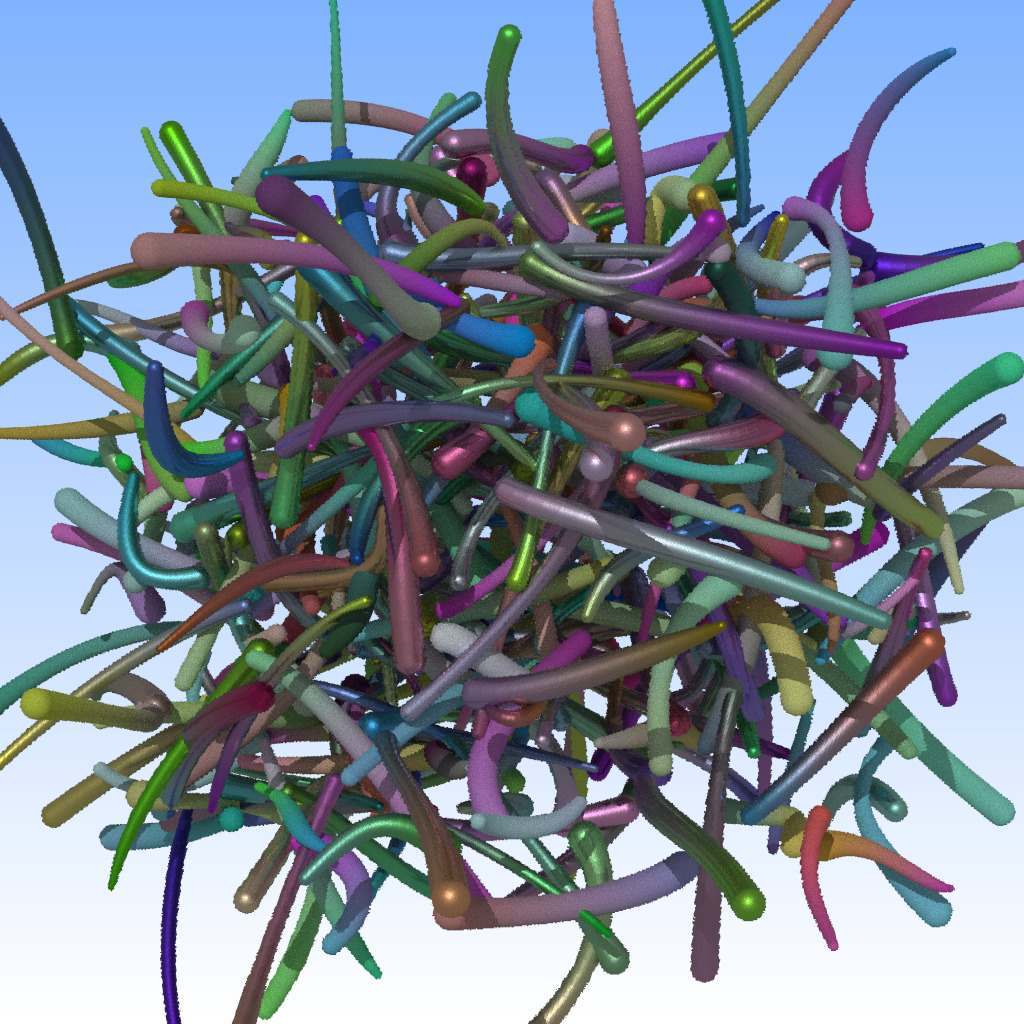
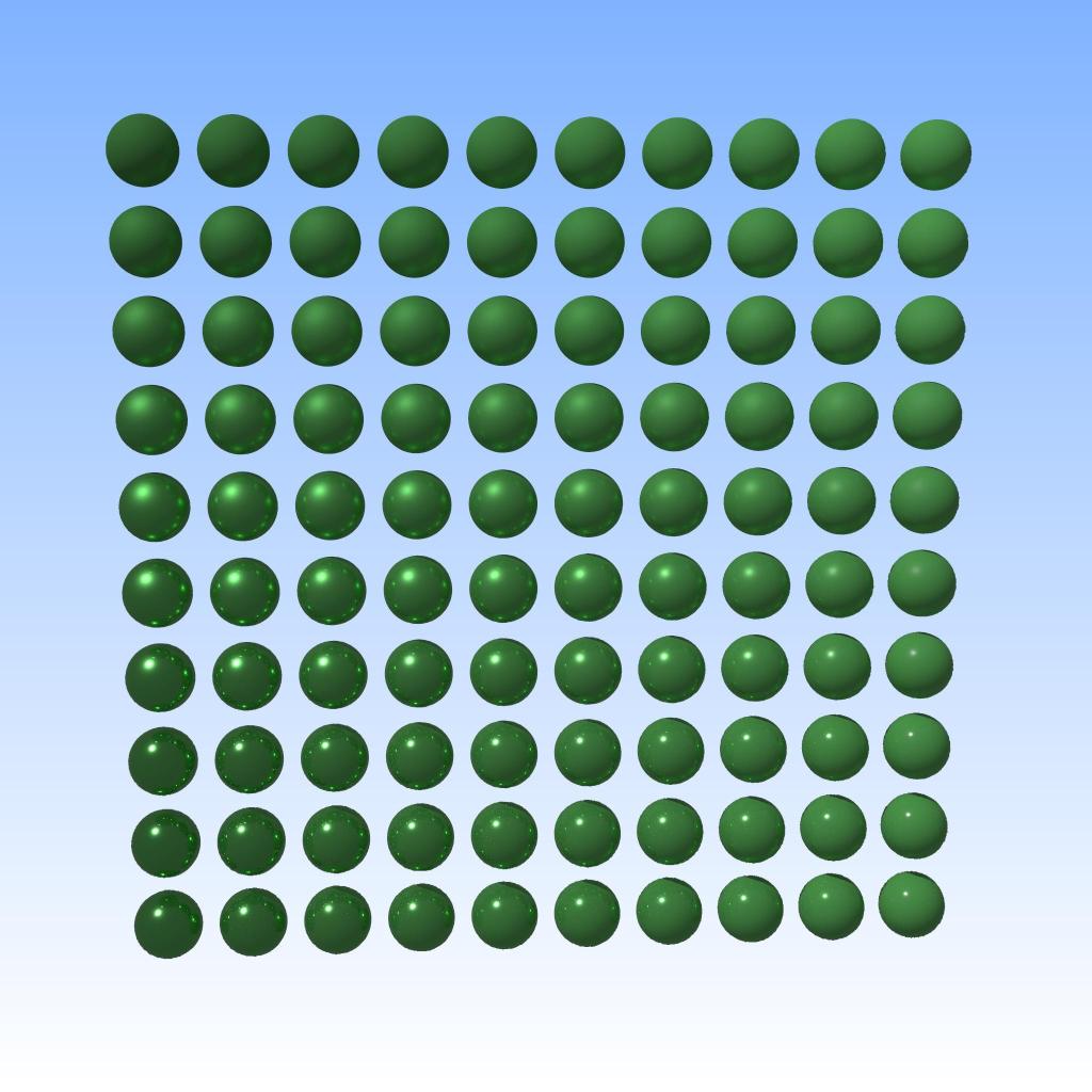
And finally, just some eye-candy to how what it can do (these are simply the samples from the pynari github repo):

(Note that the data-parallel MPI example – the fancy-colored cube of cubes – will not currently support MPI on the pip-installed package, you’d have to build the module locally for that).

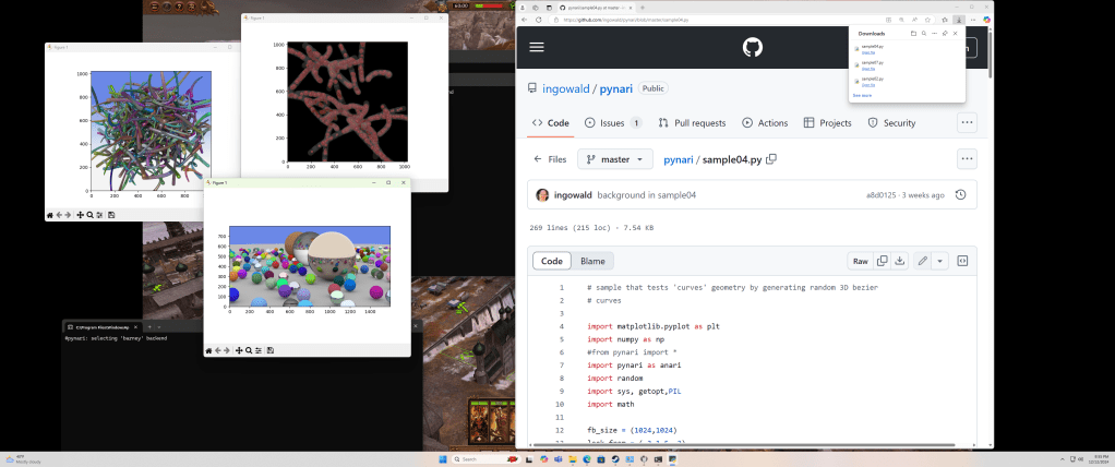
And finally, to show that it really works even on Windows (the Linux part is always a given for anything that I have written…), here a screenshot I’ve taken last night after the buildwheel finally ran through:

(the careful observer will notice Warhammer running in the background – I literally just ran that on the gaming machine my son was just playing on, and it worked out of the box!).

Kudos

Last but not least, a few kudos for those without whose help this wouldn’t have been possible:

  • Wenzel Jakob: pynari internally makes heavy use of Wenzel’s amazing “pybind11” library (https://github.com/pybind/pybind11). Thanks to pybind, the actual python bindings were – by far – the least of the problems in building this.
  • Jeff Amstutz and anybody else behind the ANARI_SDK (https://github.com/KhronosGroup/ANARI-SDK): pynari doesn’t directly use the ANARI SDK – only barney does – but those folks were incredibly helpful in fixing things that were required to make barney work in pynari (such as building static libraries).
  • Jeff Amstutz and Stefan Zellmann – not involved in pynari itself (yet?), but without those two barney would never had an ANARI interface to start with, and without barney-anari pynari wouldn’t exist.
  • Nate Morrical, from whose NVISII project I stole a lot over the years – BRDF components, guidance on building wheels, and many other things. (and without whom I’d probably never have started to learn python in the first place).

A few links for further reading (some of those have appeared above):

New Paper Preprint: Data Parallel Ray Tracing in Object Space

(sorry for the delay, this is a bit outdated – this was apparently stuck in my Draft folder, and never sent out :-/ )

Finally …. I can share this paper.

I’m actually super-happy that this paper is finally out – I’ve now been working on this particular problem/idea – on and off – for at least seven years (the first rudimentary steps on that happened when I was still at Intel!); it just took forever to actually get it to where it really worked. Part of the reason this took so long was that the first ideas were too complicated to work well, and the project needed several different breakthroughs/heureka-moments to actually work. Another is that the project has undergone at least four complete “rewrite-from-scratch”es because I kept on finding new abstractions and cleaner ways to do things as it went (and the partitioners have been rewritten more often than that, too!). Yet another is that someway half-way through I switched from doing everything on CPUs to doing everything on GPUs, and that requires some additional re-design and re-writes, and also changed some of the parameters of what the system had to cope with – one one hand that was great because one needs way fewer nodes because one is no longer limited by tracing, shading, and texturing speed … but using GPUs also means that the memory limit is both lower and harder than on the host, and in particular, that communicating between different GPUs is a bit harder than sending some MPI messages between CPUs. In theory, MPI can send data directly between different GPUs, even with RMDA etcpp (in fact, that’s awesome tech!); and yes, I’ve seen that work in practice. The problem, though, is that setting up a system to allow that isn’t exactly trvial (to say it mildly); some Supercomputing centers etc have that (mostly) down for the kind of HPC codes that their users run, but if you think about just renting a few nodes in the cloud and compiling your own MPI …well, think again.

Anyway – the “final” breakthrough came when I finally sat down and built my own stone-soup cluster in my own basement, using lots of left-ofter hardware, some RTX 8000 cards donated for the purpose by NVIDIA, and a ton of additional parts I ended up buying …. and once I was actually able to interactively run stuff that project finally managed to get together some time late fall, and the paper finally got written by the end of the year, just in time to be submitted to Siggraph.

Now as it turns out Siggraph decided to reject it – not complaining here, just saying that I got a bit of a bad foreboding when after I tagged everybody from NVIDIA, everybody from Intel, and everybody I had recently collaborated with there weren’t that many people left that would be the kind of experts in ray tracing or data-parallel rendering you’d want to review that paper. Turns out two reviewers really liked the paper (the external ones, if I had to guesss), but two others didn’t, which apparently was enough to kill it. I’m also not going to complain about the reviews from said two reviewers (just saying that no, the paper is not about “BVH building”, and yes, even if it had been I am aware of some of the more recent papers on BVHes…. anyway, I digress). Anyway; I can also feel for these reviewers – there’s a paper you’re clearly not an expert in, you have no idea how to judge it, and in case of doubt you’d rather reject it than being afterwards asked how you could possibly have accepted that. So anyway, paper got rejected there – that threw a giant wrench into a total of three different follow-up papers that were/are already in the works, but hey, that’s the nature of the peer review process – sometimes you’re lucky, sometimes you aren’t.

After the Siggraph reject I uploaded the paper to ArXiv (https://arxiv.org/pdf/2204.10170.pdf); then resubmitted to HPG, where the reviewers were a bit more favorable to it, and where I just uploaded the final version this weekend. I could of course have already shared that paper after it was uploaded to ArXiv, but didn’t want to cause any confusion among the HPG reviewers if they read any Tweets or Blogs while reviewing the paper, so decided to wait ’til the final version.

Silly(?), Useful Tools: Generating Data for Scaling Experiments

Over the many different rendering projects I’ve done over the years, I’ve frequently stumbled – again and again – over the same problem: How to get “useful” data for doing scaling-style stress-testing of one’s software. Sure, you can always take N random spheres, or if you need triangle meshes take the bunny and create N random copies of that with random positions … but then you still quickly run into lots of other issues, like, for example: “now i added all these copies they just all overlap?!”, or “ugh, how can i create the scene such that multiple scales still make sense with the same camera for rendering?”, or “what if i want more instances rather than more triangles?”, or “what if I want to look at more ‘shading’ data like textures”, etc.

All of those questions are “solvable” (this is not rocket science), but I’m always amazed how much time I spent over the years – again and again – to write (and debug, and re-debug, etc) those mini-tests. And since I just did that again I decided that this time should be the last one… so as a result of that I did add all the features I wanted, and pushed that into my miniScene repo on github.

The way this tool works is actually quite simple, generating a whole lot of spheres (or actually, “funnies”, see my tweet on how i stumbled over those), but allowing the user to control a whole lot of different parameters that can influence things like how much instantiation vs “real” geometry, what tessellation level for the funnies (ie, triangle density per sphere), what texture resolution to use for each of the funnies, etc. In particular one can control:

  • how many “non-instantiated spheres” to generate
  • how many different kinds of spheres to generate for instantiation
  • how many different instances of spheres to generate
  • what tesselation density to use per sphere
  • what texture res to use per sphere (sphere gets its own checkerboard pattern texture)

These spheres then all get put into a fixed-size slab that covers the space from (0,0,0) to (1000, 100, 1000), with sphere radii and instance scaling adjusted such that there should always be a reasonably equal density within that slab. Note that slab is intentionally 10x less high than wide, so we neither end up with just a 2D plane, nor with something that’s a cube (where all interior geometry is usually occluded by that at the boundary).

In particular, this tool allows for easily controlling whether you want to scale in instance count (increase instance count) or triangle count (increase num non-instances spheres and/or sphere tessellation level); whether to put more triangles into just finer surface tesselation or into more different meshes, how much of the output size should be in textures vs geometry, etc.

Here a few examples:

/miniGenScaleTest -o scaleTest.mini (ie, with trivially simple default settings) generates this:

num instances : 2
num objects : 2

num unique meshes : 101
num unique triangles : 40.40K (40400)
num unique vertices : 22.22K (22220)

num actual meshes : 101
num actual triangles : 40.40K (40400)
num actual vertices : 22.22K (22220)

num textures : 101

Which with my latest renderer looks like this:

Now let’s change that to use 10k instances: ./miniGenScaleTest -o scaleTest.mini -ni 10000, and we get this:

num instances		:   10.00K	(10001)
num objects		:   101
----
num *unique* meshes	:   200
num *unique* triangles	:   80.00K	(80000)
num *unique* vertices	:   44.00K	(44000)
----
num *actual* meshes	:   10.10K	(10100)
num *actual* triangles	:   4.04M	(4040000)
num *actual* vertices	:   2.22M	(2222000)
----
num textures		:   200
 - num *ptex* textures	:   0
 - num *image* textures	:   201
total size of textures	:   204.80K	(204800)
 - #bytes in ptex	:   0
 - #byte in texels	:   204.80K	(204800)
num materials		:   200

which looks like this:

But since that scene complexity is mostly all in instances (which for “large model rendering” is often considered “cheating” let’s instead add a few non-instanced spheres as well (but let’s add more instances, too, just for the fun of it): ./miniGenScaleTest -o scaleTest.mini -ni 10000000 -nbs 100000 -tr 32 (this creates 10 million instances of spheres (each having 4k triangles), and then another 100,000 spheres that are not instances, for a total of this:

num instances		:   10.00M	(10000001)
num objects		:   101
----
num *unique* meshes	:   100.10K	(100100)
num *unique* triangles	:   40.04M	(40040000)
num *unique* vertices	:   22.02M	(22022000)
----
num *actual* meshes	:   10.10M	(10100000)
num *actual* triangles	:   4.04G	(4040000000)
num *actual* vertices	:   2.22G	(2222000000)
----
num textures		:   100.10K	(100100)
 - num *ptex* textures	:   0
 - num *image* textures	:   100.10K	(100101)
total size of textures	:   1.64G	(1640038400)
 - #bytes in ptex	:   0
 - #byte in texels	:   1.64G	(1640038400)
num materials		:   100.10K	(100100)

(and zooming in a bit)

(note the “artifacts” on some of those spheres are intentional – they’re “funnies”, not spheres. I find these funnies more useful as testing geometry, but of course, if you want to generate “non-funny” spheres there’s a flag for that as well).

Now finally, let’s use this to push my two RTX8000 cards to the limit, and do this: ./miniGenScaleTest -o /slow/mini/scaleTest.mini -ni 10000 -nbs 2000000 -tr 32 … with which we end up at a whopping 800M unique triangles and an additional 32 GBs of texture data:

num instances		:   10.00K	(10001)
num objects		:   101
----
num *unique* meshes	:   2.00M	(2000100)
num *unique* triangles	:   800.04M	(800040000)
num *unique* vertices	:   440.02M	(440022000)
----
num *actual* meshes	:   2.01M	(2010000)
num *actual* triangles	:   804.00M	(804000000)
num *actual* vertices	:   442.20M	(442200000)
----
num textures		:   2.00M	(2000100)
 - num *ptex* textures	:   0
 - num *image* textures	:   2.00M	(2000101)
total size of textures	:   32.77G	(32769638400)
 - #bytes in ptex	:   0
 - #byte in texels	:   32.77G	(32769638400)
num materials		:   2.00M	(2000100)

The result looks like this:

… and just to show that this is really about to push my GPUs to the limit (even with my latest data-parallel multi-GPU renderer) here also the output from nvidia-smi:

Guess I might have squeezed a bit more (some 3GBs still unused on each GPU!), but the goal of this exercise was to have something that can bring my renderer to its limits, and guess that’s pretty much it for now.

BTW: The result still runs at 17 fps 🙂

If you want o have a look at this tool: have a look at the miniScene repo, then tools/genScaleTest.cpp. The resulting .mini file should be trivial to read and use for your own stuff, so …. enjoy!

Parallel/GPU-based Construction of Left-Balanced k-d Trees

Similar to the article I wrote last week on stack-free k-d traversal (see here), this post is about a “left-over” from many years back – one that I’ve been using on-and-off for ages, but never found the time to actually write up and share.

Well, as the very existence of this post may give away I actually did find the time to finally write this up and share it (and man, does it feel good to finally get this off my stack, after a few years of that pressing on me!). If you’re interested: the write-up is on my usual publications page (https://www.sci.utah.edu/~wald/Publications/), as well as on ArXiv (well, it will be there once it actually finishes processing – by Friday, if the email I just got is to be trusted). In addition, there’s also sample code in the github repo that I created for the reference implementation, see here: https://github.com/ingowald/cudaKDTree .

If you’re working with k-d trees (the left-balanced sort, that is), and need a GPU-accelerated way of building them, have a look. I’m not claiming this to be the un-doubtedly fastest way you could ever build a left-balanced k-d tree on a GPU (in fact, I’m fairly sure that faster methods exist, ahem), but what I really, really like about this particular method is what I’d call the the “soft metrics” of ease of use and simplicity – it’s all a pretty simple CUDA update kernel (that literally fits into a single laptop screen!), plus a bit of parallel sort… easy to use with/update for/template over different data types like int2, float3, float4, structs-with-payload (eg, photons in photon mapping), etcpp, and can be used in a header-only way, too. I’ve now used this method several times, and unlike for some other methods I have it was always trivially simple to just drop this in and use it.

The weakest part of that algorithm is that – at least for the reference implementation – I used thrust::sort for sorting, and since I need to use a custom sort operator that does fall back to a relatively slow implementation of sorting, and to one that actually needs a roughly 2x memory overhead during sorting. Both of that could, of course, be fixed by doing a better swap-based sorting via bitonic sorting … but “that is left as an exercise to the reader” :-).

Enjoy.

Stack-free k-d Tree Traversal

Yes, I haven’t written anything on this blog in a while – been too busy coding and already way overdue writing things up in latex/paper form – but since I finally managed to finally finish the write-up for that technique (which by now was overdue for now several years!) I thought I’d celebrate that milestone by at least dropping a note on that technique here, in case it’s useful for others, too….

The technique I’m referring to is a stack-free traversal method for k-d trees – and to be specific, I mean the kind of k-d trees that encode k-dimensional data points https://en.wikipedia.org/wiki/K-d_tree, not the ray tracing-related ones I used so much in my early days of ray tracing research… The algorithm is actually super-simple once you think it through – a write-up in “paper”-form (i.e., with full explanation of how it works) can be found here https://arxiv.org/abs/2210.12859; in addition, if you’re somebody that prefers header-files over PDFs you can also find some sample code here: https://github.com/ingowald/cudaKDTree. The repo that the latter link points to also contains some pretty neat GPU-friendly and parallel builder for left-balanced k-d trees, too (which is arguably even more interesting than the traversal…) … but that’s the topic for another post if and when I ever finish the write-up of that technique (in another few years!?).

Now what’s so interesting about this technique? First, it’s simple, which is always good; but more importantly, it allows you to traverse k-d trees (for photon mapping, point data, p-kd trees, etc) without needing a stack. It’s not necessarily faster than stack-based techniques (and if memory is not a concern a good BVH is almost certainly faster than a k-d tree, anyway), but in my experience on a GPU stacks always come with some strings attached, so I’ve come to now default to this technique if and when I ever need to use a k-d tree. The samples I added to this repo are intentionally small and self-contained; you can use the same technique for other queries, other dimension and data types (templates are your friend…), etc; but I wanted to keep that repo small – feel free to send PRs with other use cases if you have any to share.

With that – have fun!

PS: Again:

EGPGV Paper Talk on AMR Streaming with ExaBricks EGPGV Paper Talk on Streaming

Just back from Rome, where Stefan gave a talk on our latest paper on how we extended our “ExaBricks” AMR rendering project to allow for efficiently streaming animated AMR data.

And as there’s always a lot more involved in such a project than you could seriously put into a paper he also just wrote a very nice blog post on all the “extra” stuff that’s not in that paper. I actually thought of doing the same, but he beat me to it …. anyway: check it out here!

“Ray Tracing Massive Models using Hierarchically Compressed Geometry” – or: Huh, the things you find when sifting through your old stuff…

Sometimes you just “stumble” over things from the past that you had mostly forgotten about (or “gone into denial over”!?) …. in this case, I was sifting through my back-then-when backups for a copy of some of the large scanned models that I have previously worked with in the past (like the David, Lucy, Atlas, etc). Now my trusted find tool eventually did find some matches on my 12TB backup server, but they were png files in an old paper repo from my TACC account backup … and since I couldn’t immediately place the name of that paper repo I started to get curious, so pulled out that directory, and looked inside. What i found what this here – a “aborted” but almost-finished paper draft:

Now this draft was never actually submitted anywhere, and the style file is wrong, too (it was not submitted to EG06; in fact it wasn’t even written until around 2010 or 2011)… but still, some pretty cool ideas in there for the time – mind that this is over a decade old by now. Some of the ideas that this already talked about (in 2011-ish!):

  • a method of encoding large meshes with only 5-8 bytes per triangle including the BVH
  • using the concept of “quads” (triangle pairs with a shared edge, not necessarily planar) throughout everything, even for regular triangles; which not all ray tracers do yet even today
  • automatica generation of such quads from input triangle meshes
  • hierarchical encoding of both geometry and acceleration structure; basically the same of what we used in our 2021 paper on GPU volume ray tracing compressed unstructured mesh data sets. (And while I’m on that topic: a huge shout-out to Ben Segovia and Manfred Ernst, though, which pioneered this with their way under-appreciated Memory Efficient Ray Tracing with Hierarchical Mesh Quantization paper!)
  • a Quad-BVH with hierarchical encoding of the children relative to their parent node; similar to Carsten’s Compressed-Leaf BVHes paper from 2018
  • first interactive ray tracing of billion-plus sized models on fixed-memory “GPUs”; in this paper I used the “Phi” GPU equivalent that intel had at the time (either KNF or KNC, I really don’t know any more). Using that hardware that “may or may not” have been the reason this paper never got published at the time – but I digress.
  • first SPMD ray tracer / path tracer (RIVL) written with a predecessor/sister-project to what later become ISPC – think an ISPC-based path tracer all running on that KNx architecture.
  • an out of core streaming framework for large data (for the construction), that could even do out of core SAH construction etc, with on-the-fly compressed triangle streams etcpp (I still use that same technology today, just a different implementation).

Sigh. So much cool stuff, and all of that over a decade ago … and really cool results (<10 bytes per triangle, including BVH!) … and then I had completely forgotten about it.

Anyway …. just thought I’d drop that draft here; maybe it’ll inspire somebody to pick up some of these ideas, and do something cool with it – the paper does have some few missing text pieces, and in particular several blank tables with performance data – but the latter is actually a good thing: I didn’t do this intentionally for this blog post (I’m not even sure I still have the latex sources for that paper?!); but I would actually have somehow stripped them, anyway, so it’s good they’re not in there. That doesn’t mean that I didn’t have this running at the time (I did), or that it didn’t perform well (oh yes, it did; absolutely) …. but whoever was going to pick up on these ideas would have to re-implement that all on more modern hardware, anyway (and yes, that would probably just scream on a 3080!).

So; if anybody wants to go for it and re-investigate these ideas: feel free – I won’t do it, because I don’t have the time; but if somebody is looking for a student project, a master’s or bachelor’s thesis, or anything else of that sort, then this might still suit – and might still produce a paper, too, depending on results. And if or when somebody wants to do this on a GPU, and wants to chat about how to best do that – I can still chat, I just won’t write the code, or a new paper.

The things one finds in old accounts, indeed…

Parallel BVH Construction

Now this is a new one : usually I use this blog to write about newly published papers, or share some experience with some currently ongoing projects – but this one time, I’ll actually use this blog to direct attention back to some papers that actually happened a looong time ago. Reason: I recently had several discussions with people about the topic of fast, parallel BVH construction, and always replied by “just read that paper I wrote about that; I still use the same techniques as in my paper from 10 years ago, just with a GPU rather than a CPU” …. only to get long stares because whoever I talk to then often doesn’t know what the heck I’m talking about.

That confused me a while, until last week I actually tried to google this handful of papers that I had so vividly in my mind … and realized I couldn’t actually find them myself, because google just didn’t find what I was looking for. Now as it turns out, I’m not so delirious that I was imgining any papers that I never wrote – but unfortunately, when I wrote those papers I didn’t know how the lingo in ray tracing would eventually evolve, and apparently ended up picking paper titles that google just doesn’t match to those keyword you were probably search for: What I (naturally) googled for was “parallel bvh construction” (and if you reach this page, that’s probably exactly what you did, too) … but back then when I wrote the paper, I didn’t know that this would be the terminology everybody nowadays uses, and used different terms.

Parallel BVH Construction

So, if you are interested in parallel BVH construction (hopefully on a GPU, nowadays), I’d like to point your attention (and hopefully, google’s search algorithms) to the following two papers: First, the first one I did that actually looked at parallel construction (on a brand new “Clovertown” CPU back then, with four(!) hardware threads!) was “On fast Construction of SAH-based Bounding Volume Hierarchies“. Funnily even the web link contains the terms “parallel” and “BVH”, but the title itself contains neither, so google – at the time of this writing – really doesn’t want to find it. But if you are interested in some of the very first approaches to building SAH BVHes in parallel, this is the one – today I’d use CUDA kernels, of course, and way more threads – but the core concepts are the same. Interestingly, if you look at section “4.2. Grid-based Binning” that’s actually just a different name for what nowadays you’d call a Morton pre-binning step (well, it’s a bit more general because Morton codes are power of two, and that grid is not – but the core idea of an initial pre-binning, with an implicit BVH over those bins and a second BVH building step inside those bins, that’s the same …. but I digress).

Second, a more real-time implementation of that was done a few years later, at the time on the “MIC” Many-Core Knights-Series of Intel CPU in the following paper: Fast Construction of SAH BVHs on the Intel Many Integrated Core (MIC) Architecture. That one is a bit more specialized because it really targeted those certain chips that Intel was doing at the time (bonus assignment for the advanced graphics geek: try to guess what the “LRB” in the URL may refer to…), but it’s also still relevant because this was the first one to really target real-time re-builds, and really had to look at all these things like having lots of parallel threads (just like a GPU today), at having wide “SIMD”, etc – in fact, what I do in my latest builders on a GPU is very similar to what this paper does except that today you have “warp parallelism” instead of “SIMD” for the SAH evaluation, and you you have CUDA async task launches where this paper talks about a hand-crafted tasking system. So, if you’re really into that topic, might be worth reading, too.

Refitting BVHes and Two-Level BVH Structure

Finally, once we are on the topic of (re-)building BVHes, two other papers come to mind: The first one where we proposed the idea of BVHes for real-time ray tracing – and in particular, of using refitting – was Ray Tracing Deformable Scenes using Dynamic Bounding Volume Hierarchies (again, no “BVH” in the title, nor “refitting” – I really suck at picking well-google’able paper titles); and the first paper that proposed the idea of two-level hierarchies with a top-level acceleration structure (TLAS) and botom level accels (BLASes) – back then, still using kd-trees instead of BVHes – was Distributed Interactive Ray Tracing of Dynamic Scenes … that actually also talks about “distributed” because that was the only way to get enough compute for real-time ray tracing back then when; but it’s actually about the two-level accel structure more than it is about the “parallel rendering” component.

Real-time BVH Builds Today

Now today, times have obviously changed, and for most of the time you can probably rely on the BVH builders that come with OptiX or DXR. But from time to time one still needs to have a BVH to traverse in one’s own traversal code (maybe for searches other than tracing rays?). If I “were to go about writing a real-time CUDA builder today, I’d follow the same basic ideas as above, but obviously using GPUs and CUDA for it: One useful technique is still the pre-binning described in the first paper; and/or a two-phase build where a first stage has all threads (across all SMs) work together on splitting individual, large subtrees until they reach a certain size; then a second stage where different SMs (or different warps) work on a different subtree each; with warp-parallelism (ie, 32 threads executing the same SAH evaluation in parallel). Getting the memory allocations right requires some care, as does the proper stream handling to keep the GPU busy – but the base idea is still exactly the same … and still works like a charm. Don’t have any code to share as of right now, unfortunately; but the base ideas are right there. Have fun!

New paper preprint: “A Memory Efficient Encoding for Ray Tracing Large Unstructured Data” (aka “the ‘bigmesh’ paper”), IEEE Vis 21

TL/DR: After having worked on this on and off for now roughly three years, our work on ray tracing really(!) large unstructured data on GPUs has finally been accepted at IEEE Vis; preprint here:

Short story long: This particular paper is part of a larger project that all started when NASA first released the Fun3D “Mars Lander Retropulsion Study” data at https://data.nas.nasa.gov/fun3d/ (with a HUGE “thank you” to Pat Moran for helping to get this data out into the community: Pat, we all owe you one!). This NASA project was about using supercomputing and numerical simulation (using NASA’s “Fun3D” solver) to simulate how a capsule entering Mars’ atmosphere could use “reverse” thrusters to slow down…. and generated a truly tremendous amount of data: The simulations were performed on three different model resolutions (each being a unstructured mesh with mostly tets, but also some wedges and hexes). The fun part: even the “smallest” version of that unstructured mesh was bigger than anything else I had been able to lay my hands on at the time, and the largest one having a solid 3 billion-ish unstructured elements (billion, not million)…. plus several different scalar fields, and many, many time steps.

Just downloading this data initially took me several weeks’ work, with initially a multitude of shell scripts to get all the files, check for broken data/interrupted connections, etcetc (that process has much improved since then…); and I also had to marshal quite some hardware for it, too: over the course of this project I not only got a whole stack of 48GB RTX8000 GPUs (from NVIDIA), I also bought – explicitly for this purpose – something on the order of about terabyte of RAM to upgrade two or three machines we used for data wrangling; and built two new RAID NASes (one 12TB, one 8TB) to deal with the resulting data.

On the software front, the effort to deal with this model was, if anything, worse: though we had plenty code to build on from some previous papers on tet-mesh point location and unstructured-mesh rendering, these codes initially were totally inadequate to deal with this scale of data – no matter how well a given piece of software works, once you throw something like two to three orders or magnitude larger data sizes at it you’ll find “where the timbers start to creak”. Well, that was the whole point of looking at this data, i guess…

Eventually, looking at this data quickly turned from “oh, a new data set to play with” to what turned into a major effort where pretty much each and every one of the tools we had been using before had to be completely rewritten to better handle data of that size; and where we ended up having to go into a whole lot of totally orthogonal directions that each had their own non-trivial challenges: building tools for even interfacing with unstructured meshes of that scale (our umesh library), different approaches to render it (with sampling vs tet/cell marching, different space skipping methods, different (adaptive) sampling methods, etcpp), with lots and lots of new helper tools for stitching, for computing mesh connectivity, iso-surfaces, shells, tetrahedralizations, partitionings, ghost-cells/regions, etcpp; a new framework for data-parallel rendering that can deal with this sort of data (where, for example, individual partitions aren’t convex), and so on, and so on, and so on….

What we realized at some point was that trying to write “one” paper about all of that simply wouldn’t work: there’s far too many individual pieces that one needs to understand for the others to make sense, and just not enough space in one paper to do that. So, to focus our first paper we decided to first describe and evaluate only exactly one particular angle of the whole project – namely, how far you could possibly “squeeze” the data required for a sample-based volume ray marcher operating on an unstructured mesh: given how expensive rendering this data is it was kind of obvious that we’d want to use GPUs for it – but for models of this size, the kind of algorithms and data structures we had used before were simply using (far) too much data. Consequently, one of the angles throughout this project was always to try and encode the same(!) data in a more efficient way, to try and fit ever larger parts of the data on a single GPU … until at some point we could fit all but the largest of the three versions of this data set (and even that largest one fits on two GPUs in a single workstation).

Unfortunately, even that single angle – how far you could possibly squeeze an instructured mesh and BVH to fit on a GPU (and how to best do that!) – turned into a non-trivial effort that in total we have now worked on (on and off) for over two years: part of that problem is the non-trivial amount of data wrangling, where even running one new variant of your encoding can take you another day to run through; but a totally unexpected one was just how much effort we had to put into evaluating/comparing that method. Reviewers (correctly so) asked questions like “how does that compare to tet marching” or “how does it compare to data parallel rendering” – and though these are absolutely interesting and valid questions, the problem for us was that there simply was nothing useful to compare against … so we eventually ended up having to solve all these totally orthogonal problems, too, just to be able to evaluate ours.

For example, just for something as simple as “comparing to tet-marching” you first need to have an implementation of tet-marching, so you need a tet marcher that can deal with this size of data … but before you can even start on writing the tet marcher you first need to have a tet-mesh neighborhood/connectivity information, and computing that for “several billion tets”-sized models (think hundreds of Gigabytes) isn’t exactly trivial, either …. and of course, you can’t even start computing the tet connectivity until you have a tet-only version of that model to start with, which in turn requires you to be able to robustly tetrahedralize a model with billions of mixed elements into another one with even more billions of tetrahedral elements, while properly handling bilinear quadrilateral faces etc while tetrahedralizing, etcpp … and if want to do your tet-marching in data-parallel (which you have to, because it’s too big for one GPU), then you also have to deal with partitioning, computing boundaries/”shells”, etcpp. If I include all this “extra” work required to make this paper, then there was probably far more effort required in doing this paper than in any other paper I’ve ever worked on… and with a healthy margin to spare.

Anyway; the first paper of this project is now finally “through” the reviewing pipeline, and has just been accepted at IEEE Vis 2021 (to later appear in TVCV). As said above this paper touches upon only one part of the whole project, and upon only one particular problem – one that’s an important ingredient to all the stuff around it, but nevertheless only part of the problem. A totally orthogonal aspect of that same “master project” has also just been accepted as a short paper at IEEE vis, but that’ll deserve its own blog post at some later time.

So for now: hope you’ll enjoy the above paper – it’s been a lot of work, but also a lot of fun. In case of any questions, feel free to drop me an email or leave a comment….. enjoy!

PS: Just a few of the images, to give you an idea of that data:

First, a volume rendering of the whole lander – note that there’s literally hundreds of millions of elements in that single view, and often dozens of tets per pixel (and not just in depth, but side by side!):

Now to give an idea of just how detailed the data behind this innocuous looking image is, here a is-surface that I extracted from that (yet another tool we had to write from scratch to deal with this size of data) :

Note this is for a different camera partition, but if you mirror it left-to-right you’ll probably see where they roughly match up. Doesn’t look too bad yet, because the tets (and thus, triangles) on the outside are much larger than those in the turbulent region, giving the totally wrong impression that the mesh wasn’t actually that fine: but this mesh alone is several hundred million triangles – and of course, is only a isosurface “cut” through the volumetric mesh.

Next let let’s use a color-coded version of this iso-surface, where different colors indicate some spatial pre-partitioning into blocks of already non-trivial models (remember, this is a isosurface from a volumetric mesh). As to how big each color-coded chunk is: I can’t say for sure (that image is over a year old), but I’m fairly certain those are the same as the “submeshes” we talk about in the paper, so roughly 64K vertices (maybe around 250K elements?) per chunk.

Now from that, let’s look at only the tiny region that is marked with a red square, and zoom in on that one, with the same “submesh ID” shader:

And finally, let’s take this same view, and render with a triangle ID shader to show individual triangles of this iso-surface:

Though hard to show in still images (it’s much more impressive if you can do that interactively 🙂 ), this hopefully helps in showing just how ridiculously finely tessellated this model is: each triangle you see in the iso-surface is roughly one tet in the volumetric model – except all the “whilespace” that the isosurface doesn’t show is full of tets (and other elements), too. And remember, that is only one tiny part of one plume of turbulence in the model, that in the beauty-shot above maps to just a handful of pixels… fun indeed 🙂

Time to Image: 2 Hours … :-)

If you read this title for the first time, you may be excused for wondering why I’m happy about a 2-hour “time to image”: usually “time to image” means the time it takes for a interactive renderer to get from starting to load a model to when it is ready to display the first image on screen … and anything over “seconds” is usually not all that useful. In this case, however, I meant “time to first image” in the sense of “starting with a completely blank repo, to having a interactive OWL/OptiX-based viewer that can render a model”. And in that meaning, two hours IMHO is pretty awesome!

Let’s take a step back. Why did I actually do this?

On Sunday, I finally posted a first article on OWL, which only recently got tagged as “1.0”, i.e., with some reasonable claim to “completeness”. In this article, I made a big deal about how much easier OWL can make your life if you want to write an OptiX/RTX accelerated GPU ray tracer …. but what could I actually base this claim on? Sure, I/we have by now several non-trivial OWL-based renderers that show what you can do with … but how would one actually measure how easy or productive its use would be?

While on the way to get my coffee I decided to simply run a little self-experiment – initially not to prove a point, but simply because I was curious myself: To do that, I decided I’d pick something simple I always wanted to write but never got around to (I picked a structured-volume direct volume renderer), and then spend a day or two trying to write one. Using OWL, of course, but otherwise starting with a blank repo, with no other libraries, etc…. and to keep an eye on the clock, to see where time goes while doing that.

Stage 1

Oh-kay …. how’d it go? I got home from the coffee run that gave me that idea (had only sipped at this coffee so far…), then went to gitlab, created a new blank repo, called it owlDVR. Cloned it, added submodule, created a CMakeLists.txt that is about 15 lines long, created a ‘deviceCode.cu’ with a dummy raygen program, and started on some simple host code: created a ‘Model’ class to hold a initially procedurally generated N^3 float volume, created a new windowed viewer by deriving from the owlViewer that comes with the owl samples, overrode the ‘render()’, ‘cameraChanged()’ and ‘resize()’ methods, and then started on the actual OWL code: create context, launch params, and raygen; build pipeline and SBT; upload the volume into a buffer and assign that buffer and volume size to launch params in the constructor (and of course, build pipeline and SBT); then add some owlLaunch2D() in Viewer::render() and some owlParamsSet()’s for the camera in Viewer::cameraChanged() ….. and that was pretty much it from the host side.

Then take the deviceCode.cu, and start filling out the raygen program: create a ray from the camera parameters that I put into the launch params, intersect ray with the bounding box of the volume, step the ray in dt’s through the resulting [t0,t1] interval, add a tri-linear interpolation on the buffer holding the volume data; put the result into a hand-crafted procedural “transfer function” (pretty much a clamped ramp function), and get this (and of course, you can interactively fly around in this):

Not really super impressive as a volume renderer per se …. but finally looking at the clock, the whole project took slightly less than two hours, on nothing more than a laptop, while sipping a cofffee. And full disclosure: these two hours also include helping my son with some linear-algebra math homework (yes, covid-homeschooling is just great…).

Of course, I’ve now written a ton of other OWL samples myself, so I’ve gone through the motions of creating an OWL project before, and knew exactly what to do – somebody that’s never done that before might take a while longer to figure out what goes where. However, this still surprised myself about just how quickly that worked – after all, this is not just a simple blank window, but even already includes volume generation, upload, and a more or less complete ray marcher with transfer function etcpp … so the actual time spent on writing OWL code is even way less than that – and that surprised even me.

Stage 2: Fleshing it out

After this “first light” was done, I did spend another two hours fleshing this sample out a bit more: first adding CUDA hardware texturing for the volume and the transfer function, then later some actual model loaders for various formats, and some prettier shading via gradient shading …. all of which took another two hours, which were roughly spent in equal times on

a) creating textures, in particular the 3D volume texture : the transfer function texture was simple, because OWL already supports 2D textures, so that was trivial; the volume texture I had to first figure out how CUDA 3D textures even work, which took a while.

b) creating the actual transfer functions and color maps – I liberally stole some of Will Usher’s code from our exabricks project for that, but then spent half an hour in finding a bug in re-sampling a color map from N to M samples. (I guess the coffee had worn off by that time :-/ ).

c) adding loaders, fleshing out float vs uint8 format differences, adding gradient shading, etc.

All together that second stage took another two hours (and in that case this does include the time to help our “tile guy” unload his truck for our bathroom remodel…). Here some images that show the progression of that second stage: left the original first-stage volume with a simple hard-coded ramp transfer function and manual tri-linear interpolation; then the first picture with CUDA textures and a real color map in the transfer function; then after adding a loader for the 302^3 float “heptane” model, and on the right, after adding uint8 volumes and adding gradient shading, with the 2048^2×1920 LLNL Richtmyer/Meshkov-250 model (I had to move to my 3090 for the latter – laptop didn’t have enough memory).

The main thing I haven’t added yet is a real transfer function editor widget, and of course, as with any GUI code that may well end up taking more time than all the above combined… but as a “proof of concept” I’d still argue this experiment was quite successful, because the one thing that I did not have to spend much time on in the entire project was anything involving OWL, SBTs, programs, buffers, etc.

One valid question that any observant reader could raise is that in this sample I didn’t actually use anything that really required RTX and OptiX – I did not create a single geometry, and could have done the same with just plain CUDA. This is true (obviously), and in retrospect I might have picked another example. However, adding some additional lines of code to create any triangle meshes at this point would indeed be trivial, and would almost certainly take less than 5 minutes… In fact, I might do just that for adding space skipping: all I’d need is creating some rough description of which regions of the volume are active, then I could trace rays against that to find entry- and exit-points, and done.

Where to go from here?

As mentioned above, this little experiment started as a little exercise in “I want to know for myself”; and the main motivation for this blog post was to share that experience. However, literally while writing this blog I also just realized how useful it would be for for some users if I documented the individual steps of this toy project in a bit more detail, ideally in enough detail that somebody interested in OWL and/or OptiX could follow the steps one by one, and end up with something that would be “my first OWL / OptiX program, in less than a day”….. That would indeed make a lot of sense; but that’ll to wait for another post…